
Window Functions – Part Two
Authors: Yoav Shimonovich – BI solution expert
overview
in the second part of the article, we are going to discuss analytical functions and how we can apply their unique functionality to help us solve various scenarios.
analytical functions can be divided into two groups:
- ranking functions – this group generates a series of numbers to rank rows within its partition.
- value functions – this group allows you to compare values from previous or following rows within its partition.
| ranking functions | value functions |
| row_number | lag |
| rank | lead |
| dense_rank | first_value |
| percent_rank | last_value |
| n_tile | nth_value |
as shown in the table above, each group contains five analytical functions (at the current moment this article is being written in April 2022). however, we are going to discuss only three of the functions above which are among the most commonly used:
- row_number
- rank
- lag/lead
row_number
let’s take another look at our sales table:
( below is the script for creating the sales table. the queries are running on sql server but can be executed on any platform. you can skip this part if don’t wish to run the code on your local environment).
if you haven’t yet read the first part of the article – click here
create table sales
(
category varchar(25),
[date] date,
sales int
)

insert into sales values
('electronics','2021-08-18',1617),
('furniture','2021-11-09',1532),
('clothing','2021-11-27',1060),
('clothing','2021-08-18',1617),
('clothing','2021-08-08',1618),
('clothing','2021-11-25',1661),
('office supply','2018-06-29',815),
('office supply','2021-12-20',3696),
('furniture','2018-10-30',844),
('furniture','2021-12-04',1747),
('electronics','2020-11-23',4377),
('electronics','2020-10-16',1115),
('electronics','2021-08-17',3786),
('electronics','2021-10-17',1423),
('electronics','2020-09-23',4331),
('electronics','2018-12-15',3144),
('electronics','2019-07-11',1180),
('electronics','2021-10-14',3499),
('electronics','2019-09-20',406)
select * from sales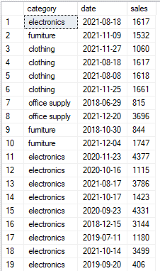
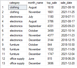
suppose that you are the manager of the store and you want to see all the top sales by month and by category.
in this example, the table is rather small and you could use traditional group by clause to solve this:
select category,
datename(month, date) as month_name, max(sales) as top_sale
from sales
group by category, datename(month, date)
order by category,  month_name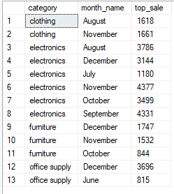
but, what if you wanted to see the full date of the sale and not just the month name?
or what if the table was larger and contained more descriptive columns that needed to be seen in the output? it is possible to use the group by clause, but when a large number of columns are added to the grouping, it gets very uncomfortable writing and reading the query. additionally, you can sometimes lose the aggregation level you desire.
a classic way of handling the task would be writing a cte:
with group_tab as
(
select category, datename(month,date)as month_name, max(sales) as top_sale
from sales
group by category, datename(month,date)
),
date_tab as
(
select sales, date as sale_date
from sales
)
select gt.category,gt.month_name,gt.top_sale,dt.sale_date
from group_tab gt join date_tab dt
on gt.top_sale = dt.sales
order by category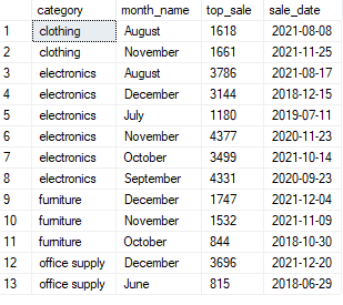
again, the end result is good, but the code is a bit long and clumsy to write.
we can use the exact same result using the row_number function:
with tab_1 as
(
select *,
row_number() over(partition by category, month(date) order by sales desc) as rn
from sales
)
select category, datename(month,date) as month_name ,sales as top_sale, date as sale_date
from tab_1
where rn = 1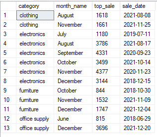
much shorter, simpler, and more flexible code!
the row_number function generates a series of numbers and orders them ascending or descending as one sequence or several sequences – according to the number of partitions.
unlike window aggregators, analytical functions must have an order by clause which determines the sorting order of the output.
select *,
row_number() over(partition by category, month(date) order by sales desc) as rn
from sales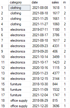
as seen from the first part of the query above, the row_number functions generated a series of numbers starting from one in each partition and ordered them by the sales amount in descending order.
going back to our table – imagine that we change one of the sales and date column values so that we have duplicated values as follows:
update sales
set sales = 1618 where date = '08-18-21' and category = ‘clothing’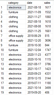
now, if we try the previous solution – it will be incorrect because we have two values of 1618 in rows 4 and 5 instead of just one, and both of them should appear:
how should we solve this problem?
rank
the rank function is very similar to the row_number function: it generates a series of numbers. but unlike row_number it uses logic to rank them and not just orders them ascending or descending.
select *,
rank() over(partition by category, month(date) order by sales desc) as rank
from sales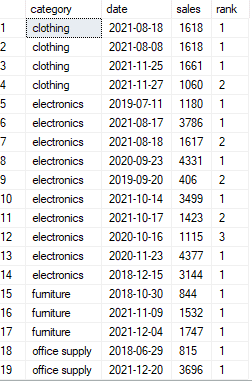
as you can see from the table above, when there are ties in the sales column – rank will give both of them the same value – in our case, it would be number one.
so if we try the full solution now, it should be working:
with tab_1 as
(
select *,
rank() over (partition by category, month(date) order by sales) as rank
from sales
)
select category, datename(month,date) as month_name ,sales as top_sale, date as sale_date
from tab_1
where rank = 1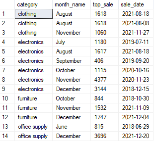
very clean, flexible, and elegant solution!
lag/lead
imagine that your supervisor has asked you to compare the sales of each department with the previous sale and calculate the percentage difference between them.
with the help of the lag function we can do it in an easy manner:
if you haven’t yet read the first part of the article – click here
select *,
lag(date, 1) over(partition by category order by date) as previous_sale_date,
lag(sales, 1) over(partition by category order by date) as previous_sale
from sales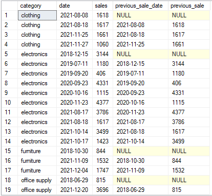
the lag and lead functions take two parameters – the column name that you want to compare values against, and the number of rows before(lag) or after(lead) the current row to compare to. in our case, we just need the previous last sale, so the value is one. as seen in the table above, some of the rows contain null values – because they are the first sales of the category and there are no previous values to compare them to.
now we can easily calculate the percentage difference:
with tab_1 as
(
select *,
lag(date, 1) over(partition by category order by date) as previous_sale_date,
lag(sales, 1) over(partition by category order by date) as previous_sale
from sales
)
select category,date,sales,
isnull(cast(previous_sale_date as varchar), 'first category sale') as last_sale_date,
isnull(cast (previous_sale as varchar), 'first category sale') as last_sale_price,
isnull(format(1- (cast(sales as float)/previous_sale), 'p'),'0.00%') as [%_difference__from_last_sale]
from tab_1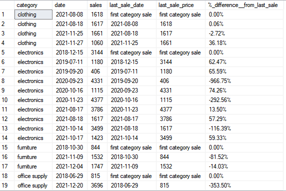
nice and clean!
conclusion
as you can see, analytical functions can be a great essence to solving different analytical problems, and it is recommended for everyone who is using sql to perform data analysis to learn them.
however, the above cases are just a brief introduction to the subject, and for the avid reader, we recommend further exploring the topic.
an important note: this article didn’t discuss the performance part of window functions.
when working with large datasets, performance is a very important part of query efficiency. therefore, before choosing any method of work, we recommend considering its pros and cons and make an educated decision based on your organization’s requirements.
nice!
hope you enjoyed the article, in the next part we are going to discuss analytical functions and their applications.
an important note:
this article didn’t discuss the performance of window functions. when working with large datasets, performance is a very important part of query efficiency. therefore, before choosing any method of work, we recommend considering its pros and cons and make an educated decision based on your organization’s requirements.
Click here to read the previous part of the article: Window Functions – Part One