Window Functions – Part One

Authors:  Yoav Shimonovich – BI solution expert

overview

Window functions are a set of functions that were introduced in 2003 and can be used to solve a variety of scenarios in analytics. Their big advantage over other methods is their great flexibility.
window functions allow you to perform both basic and complex calculations over the entire table, but unlike standard aggregate functions that have to be used at the granularity of the group level, window functions can be used in the granularity of the row level as the next illustration shows:

window functions can be divided into two main categories (some divide into more, but for simplicity reasons, we will stick with the letter):

• window aggregates.
• analytical functions.

because each category deserves its own introduction, the first part of this article will be about window aggregates, and the second part will discuss analytical functions.

window aggregates
let’s take a quick look at our sales table (below is the script for creating the sales table. the queries are running on sql server but can be executed on any platform. you can skip this part if don’t wish to run the code on your local environment).

create table sales
(
category varchar(25),
[date] date,
sales int
)

insert into sales values
('electronics','2021-08-18',1617),
('furniture','2021-11-09',1532),
('clothing','2021-11-27',1060),
('clothing','2021-08-18',1617),
('clothing','2021-08-08',1618),
('clothing','2021-11-25',1661),
('office supply','2018-06-29',815),
('office supply','2021-12-20',3696),
('furniture','2018-10-30',844),
('furniture','2021-12-04',1747),
('electronics','2020-11-23',4377),
('electronics','2020-10-16',1115),
('electronics','2021-08-17',3786),
('electronics','2021-10-17',1423),
('electronics','2020-09-23',4331),
('electronics','2018-12-15',3144),
('electronics','2019-07-11',1180),
('electronics','2021-10-14',3499),
('electronics','2019-09-20',406)

select * from sales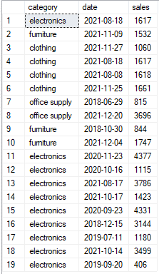

suppose that we want to calculate the total sales – we can achieve this with a simple sum aggregation:

select
sum(sales) as total_sales
from sales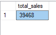

what if we would like to see the total sales of each category separately?
the group by clause can aggregate our data in the category level:

select category, sum(sales)as total_Sales_by_category
from sales
group by category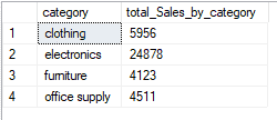

now up to this point, everything is clear and straight. but what if we would like to see the individual sales of each month and the total sales?
using the group by clause this time wouldn’t help, because we want to see the data at the row level and not at the group level.
we can, however, use a simple sub-query to achieve the desired result:

select *,
(select sum(sales) from sales) as total_sales
from sales
order by category,date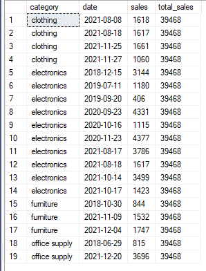

all done.
but what if we need to see the total sales by department and not as a whole?
we could do something like this:

select sales.category,sales.sales,sales.date,total_sale_by_category
from(
select category, sum(sales) as total_sale_by_category
from sales 
group by category
)grouping_table join sales on sales.category = grouping_table.category
order by category,date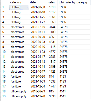

but then we begin with nested sub-queries which aren’t so comfortable reading.
we could also write a cte instead :

with sales_table as
(
select *,
(select sum(sales)from sales) as total_sales
from sales
),
group_by_table as 
(
select category,sum(sales) as total_sale_by_category
from sales 
group by category
)
select sales_table.category,sales_table.date,sales_table.sales,
group_by_table.total_sale_by_category
from sales_table join group_by_table 
on sales_table.category = group_by_table.category
order by category,date

although the end result is the same and easier to read, the code is relatively long to write.
however, we have another option – we could use window aggregates.
window aggregates act like standard aggregates, only that their result is being shown in the row level.

select *,
sum(sales) over() as total_sales
from Sales
order by category,date

using the over() clause we define our window. by leaving the brackets inside the clause empty we tell sql in the above example to treat the entire table as one window.
we can add the partition by a clause that lets us divide our current window into several smaller windows according to the partition we want – for example, the category partition:

select *,
sum(sales) over(partition by category) as total_sales_by_category
from sales
order by category,date

we got the exact same result but look at the difference in code length and code simplicity!
if we wish, we can also add the year level partition:

select *,
sum(sales) over(partition by category, year(date)) as total_sales_by_category_and_year
from sales
order by category,date

you can add as many partitions as needed with the partition by clause.
what if we want to see the percentage of each sale from the total sale by category and year?

select *,
sum(sales) over(partition by category,year(date)) as total_sales_by_category_and_year,
format(sales/sum(sales*1.0) over(partition by category, year(date)), 'p') as [%_of_total_sales_by_category_and_year]
from sales
order by category,date

you can now see the great capabilities these functions have.
this kind of calculation would be very hard (but not impossible of course) to achieve without the use of window aggregates.

the window frame
Suppose that you are the manager of the store, and you want to analyze a Pareto distribution of the sales and a moving average of the last three sales regarding the department. there is more than one way to solve this using sql, but using window aggregates is definitely the easiest one:

select *,
sum(sales) over(order by date) as runing_total
from sales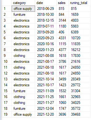

the resulting table shows that sql has calculated the running total of the sales by date.

using the order by clause, the default window frame of this clause is range between unbounded preceding and current row – meaning that sql will sum all the values starting the first row in an accumulated way till every current row. although range is the default term it is more recommended to use rows instead – there are some slight differences between the two, however, we will not discuss these differences in this article.
note that if you just want to present the sum of each category in a sorted way by date, for example, it is best to use the order by clause at the end of the query and not inside the over () clause.
you can change the window frame to perform different calculations on the rows, as the next table summarizes:

window frame type	execution on a partition
unbounded preceding	the frame starts in the first row
unbounded following	the frame ends in the final row
n preceding	a physical number of rows before the current row.
n following	a physical number of rows after the current row.
current row	the row of the current calculation

the next step in the analysis will be to calculate the accumulative percentage of each accumulative sale:

select *,
sum(sales) over(order by date) as runing_total,
format(sum(sales*1.0) over(order by date rows between unbounded preceding and current row)/sum(sales) over(),'p') as pareto_analysis
from sales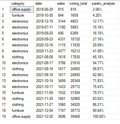

just four lines of code!
for the second part, we can use the average function with a window frame.
the window frame tells sql on which rows to look at each time when computing the calculation.
for a moving average of three sales, we need each time three rows – the current row, and the rows of the last two previous sales.

select *,
avg(sales) over(order by date rows between 2 preceding and current row) as moving_last_three_sales_average
from sales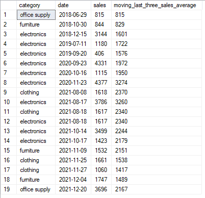

nice!
hope you enjoyed the article, in the next part we are going to discuss analytical functions and their applications.

an important note:
this article didn’t discuss the performance of window functions. when working with large datasets, performance is a very important part of query efficiency. therefore, before choosing any method of work, we recommend considering its pros and cons and make an educated decision based on your organization’s requirements.

Click here to read the next part of the article: Window Functions – Part Two